Machine Learning

Machine learning, uses data instead of human knowledge from traditional programming, and we replace hand-crafted code with a function f(x) learned from that data.

ML development has 3 stages:

• training: learning a function that explains well the training data
• test: evaluating the performance on data never seen before (generalization)
• inference: using the model in production

types of ML

• supervised learning (labeled data: given training data and output examples)
  • regression: predicting height of a dog given training data (just use y = a*x + b)
  • classification: classify cats and dogs using height+weight learning in higher dimensions (raw pixels) is harder, cant do it with classical ML
• unsupervised learning (no labels: given training data and not output examples)
• reinforcement learning (rewards from sequences of actions)

Datasets

Dataset: collection of examples (input-output mapping), each example contains a feature vector (collection of some relevant measures). Train and test samples have to be drawn independently but have to be identically distributed (from the same data generation process).

ML models

It’s a function that maps the input to the output. during training, we explore the hypothesis space (set of functions that a ml model can implement) until we find a function that explains well the data.

Objective Function

aka criterion. it’s a function we want to minimize. it quantifies how good are the predictions obtained with the learning function. often, it’s written as an average (or sum) over the training samples. empirical risk minimization: it’s the training process based on minimizing this objective.

• regression problems usually use Mean Squared Error (MSE) -> (how far are the predictions from the targeted one?)
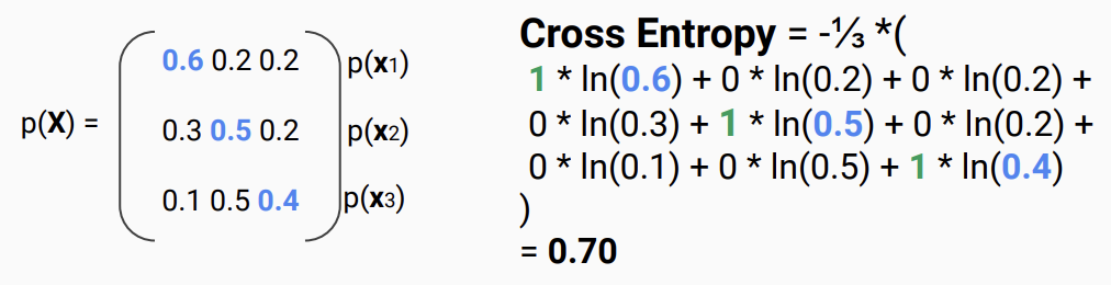
• classification problems usually use classification accuracy (N_correct / N_tot) accuracy is a “hard” metric, but ml algos prefer “soft” metrics the accuracy can be the same sometimes but the model can be more confident about correct predictions (which would be better). accuracy doesn’t catch this nuance.
  • cross-entropy (or negative log-likelihood LLN) is a softer alternative. it ranges from 0 (perfect solution) to +inf (bad solution)

Parametric Models

It can be completely described by a fixed number of parameters (in the case of NNs, by weights and biases), regardless of how much data we have.

• Linear Regression is parametric: $\hat{y} = w_0 + w_1x$ will always need two parameters to describe the models, no matter how many data points we have. Training just means finding the best values for those parameters.

• k-Nearest Neighbours (kNN) is non-parametric: to make a prediction we look at the training data directly (the neighbours), that model literally stores all training examples and uses them to decide outputs.

• $\hat{y} = f(x, \theta)$ -> running model with inputs x and current parameters $\theta$

• $\theta = [\theta_1, ..., \theta_P]^T$ -> the parameter vector, living in parameter space $\mathbb{R}^P$ (big multi-dimensional space where every point = one possible model) each unique combination of values $(\theta_1, \theta_2, ...)$ defines one possible function $f_i$

• the goal of training: find the parameters $\theta$ that make the loss $J$ as small as possible. $\theta^* = \underset{\theta}{arg\:min}\:J(Y, f(X, \theta)$) $J(\cdot{})$ = the objective (loss) function $Y$ = true labels or outputs $F(X, \theta)$ = model’s predictions for all training inputs

  For example, for linear regression, we can start with random parameters (e.g. $w_0=0$ and $w_1=1$), we could do little steps forward/backward for all the parameters and monitor how the performance changes. This little step -> gradient

Capacity

The capacity of a model tries to quantify how “big” or “rich” the model is. How many relationships can it quantify? It’s not the number of functions in the hypothesis space (that can be infinite), but rather the variability in terms of “family” of functions (can it implement linear functions only, or linear, exponential, sinusoidal, logarithmic?).

• 1-layer (few neurons) NN or a linear regression model: low capacity
• deep network or 10th degree polynomial: high capacity

Generalization

It’s the ability of a model to perform well to new, previously unseen data. It generalizes well if the test loss (objective function computed with the test set) is low.

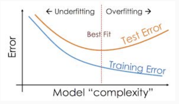
• Underfitting: when training loss is not low enough (function found by algorithm could be too simple) -> happens when capacity is too low
• Overfitting: the gap between training and test losses is too large (function found by algorithm could be too complex to explain well the training data) -> happens when capacity is too high, or not enough training examples

Regularization

Techniques aimed to counteract overfitting. It penalizes too complex models, encouraging the model to stay simple. If it has too high capacity, model can fit both real patterns and random noise in the training data (bad!).

• it reduces model variance (less sensitivity to noise)
• makes learned patterns smoother and more general
• prevents memorization of outliers

inspired by Occam’s Razor “among competing hypotheses that explain the data equally well, choose the simplest one”

• no regularization: $\theta^* = arg\:\underset{\theta}{min}\:J(Y, f(X, \theta))$ training just minimizes loss J, purely trying to fix training data perfectly
• with regularization: $\theta^* = arg\:\underset{\theta}{min}[J(Y, f(X, \theta)) + \alpha\Omega(\theta)]$ we add a penalty term to discourage overly large or complex parameter values $\Omega(\theta)$ = regularization term -> measures model complexity $\alpha$ = hyperparameter controlling how strong the penalty is if large -> care more about simplicity if small -> care more about fitting data
  • L1 regularization (Lasso): $\theta^* = arg\:\underset{\theta}{min}[J(Y, f(X, \theta)) + \alpha||\theta||_1]$ penalizes the magnitude of weights linearly (not squared) -> pushes many parameters to exactly zero, leading to sparser models (feature selection effect)
  • L2 regularization (Ridge): $\theta^* = arg\:\underset{\theta}{min}[J(Y, f(X, \theta)) + \alpha||\theta||_2^2]$ penalizes large weight values (because squaring amplifies big numbers) -> keeping all parameters small and smooth works better with gradient descent as it’s fully differentiable (L1 can be non-differentiable at 0) -> more on this later

Hyperparameters

It’s special parameters that control the learning algorithm itself (while normal parameters $\theta$ controls the ml model, being internal to $f(x, \theta)$) examples: the $\alpha$ in regularized models, learning rate, batch size, number of epochs. How to choose them? We perform training experiments with different sets of hyperparameters and choose the best one.

• BUT! We cannot use the performance achieved on the training set -> that will increase the risk of overfitting
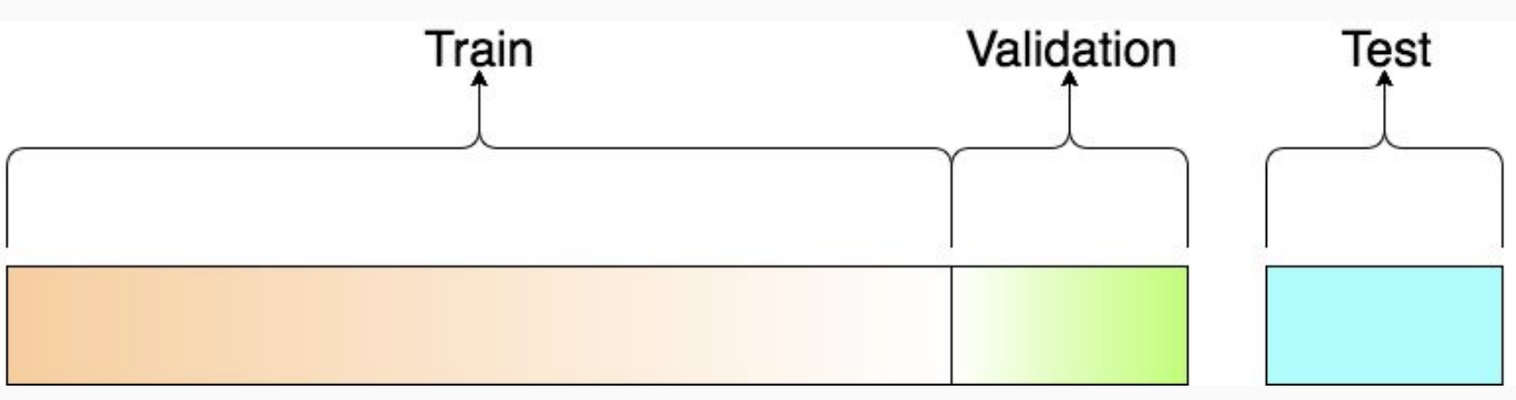
• We cannot use the performance achieved on the test set -> that will overestimate the actual performance of the system We employ a third set, validation set to choose the best set of hyperparameters. Normally extracted from training data (10%-20%)

Training set -> find best parameters Validation set -> find best hyperparameters

Searching for best hyperparameters is expensive because we have to train the model multiple times before finding the best configuration. So to optimize it we can initialize them with reasonable values. Then we fine-tune them through a hyper-parameter search:

• Manual search
• Grid search (trying different combinations)
• Random search (randomly sample hyperparameters, weirdly efficient)
• Bayesian Optimization (probabilistic guesses)

We find parameters $\theta$ with gradient descent. But we can’t compute the gradient over the hyperparameters, that’s why we use hyperparameter search. We can’t compute the gradient easily because we can’t change the hyperparameters unless we restart. We’d have to differentiate through the entire training process, possible, there’s research, but computationally massive and unstable for large models.

Deep Learning

Deep learning is a subset of machine learning which main object of study is neural networks (modular but powerful framework for creative predictive models) Machine learning uses different types of algorithms (linear regressions, decision trees, random forests, k-means clustering, etc). DL only uses NNs with many layers.

DL, with respect to ML, requires high computation power, is less interpretable as the inside of a NN is a black box, and needs large amounts of data. Also, in DL, feature engineering (extraction, selection, transformation of raw data…) is automatic.

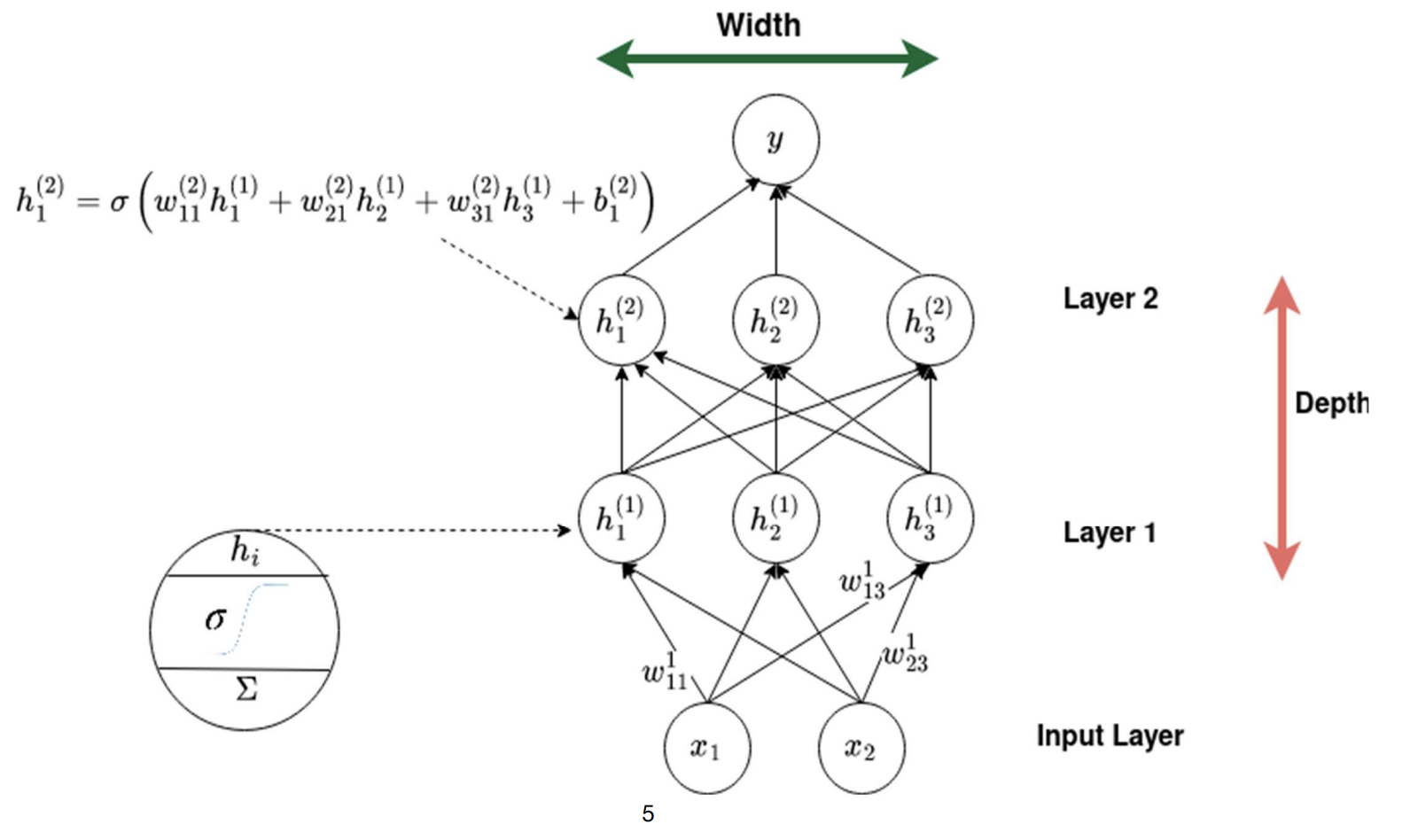
this means: weight of 1st layer, receiving neuron is #2 (next layer), sending neuron is #3 (prev layer)