Gradient Descent

It’s a technique to solve the optimization problem of Empirical Risk Minimization which just means minimizing the average loss over our dataset. $\underset{x}{min}\:\mathcal{L}(X, Y, w) = \frac{1}{N}\sum^{N}_{i=1}\ell(f(x_i; w), y_i)$

• $\ell$: loss for one sample (e.g. how wrong we are on one image)
• $\mathcal L$: average loss over all $N$ training examples
• $w$: model parameters (weights)

To minimize $\mathcal L$, we move the parameters $w$ a little bit in the direction that makes the loss decrease fastest, that direction is given by the negative gradient of the loss with respect to $w$. $w_{t+1} = w_t - \nabla_w\mathcal L(X,Y,w_t)$

• $\nabla_w\mathcal L$: vector of partial derivatives (how much each weight affects loss)
• $\alpha$: learning rate (step size)
• $t$: iteration number

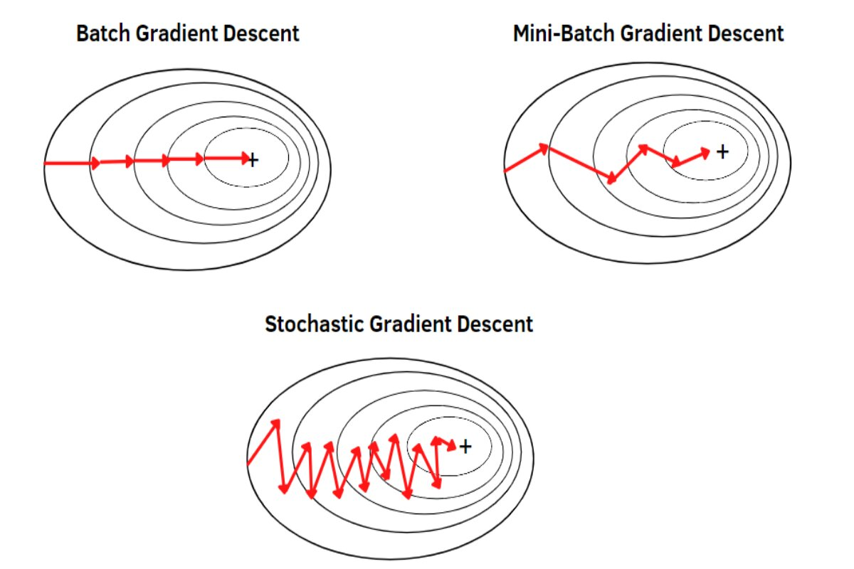
Gradient Descent Variants

• Batch (Full) Gradient Descent
  • Compute the gradient using the whole dataset
  • Precise but slow (need to pass through all samples before one update) (one update per epoch) $\nabla_w\mathcal L(X, Y, w)$
• Stochastic Gradient Descent
  • Compute the gradient using one sample at a time
  • Noisy but much faster, updates happen every time (one update per sample) $\nabla_w\ell(x_i, y_i, w)$
• Mini-Batch SDG
  • Compute the gradient on a small subset (e.g. 32 or 64 samples)
  • Faster than full batch, more stable than pure SDG (one update per batch) $\nabla_w\mathcal L(X_n, Y_n, w)$

How to compute the gradient?

Finite difference requires $O(d)$ forward passes where $d$ is the number of parameters.

• Forward difference (1 forward pass per parameter) $\frac{\partial f}{\partial w_i} \approx \frac{f(w_i+\varepsilon) - f(w_i)}{\varepsilon}$
• Central difference (2 forward passes per parameter) $\frac{\partial f}{\partial w_i} \approx \frac{f(w_i+\varepsilon) - f(w_i - \varepsilon)}{2\varepsilon}$

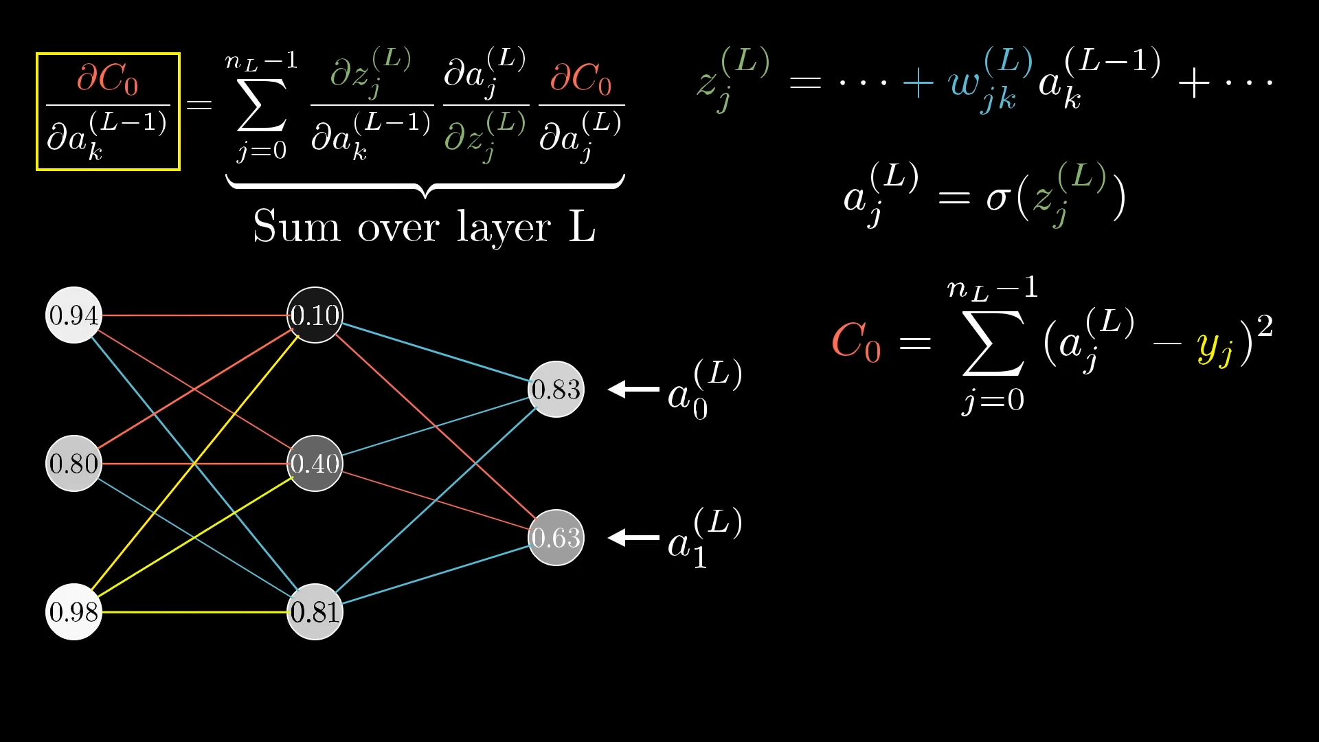
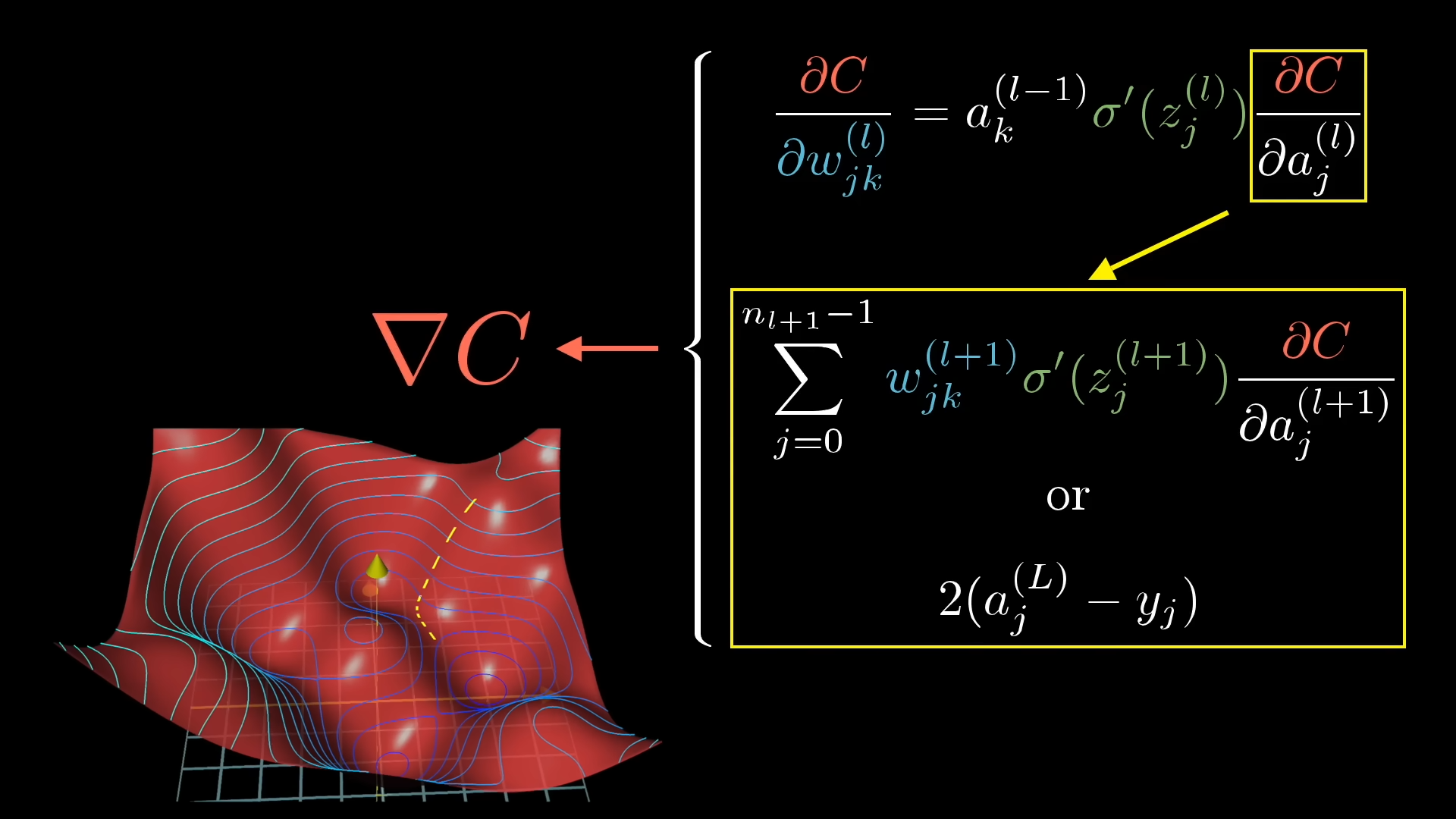
Automatic Differentiation

Much more efficient. $O(1)$ per layer. We compute derivatives exactly and efficiently by applying the chain rule programmatically.

• Forward-mode AD (compute derivatives and go forward)
• Reverse-mode AD (aka backpropagation)

PyTorch model

import torch
import torch.nn as nn
import torch.optim as optim

# Define model
class Net(nn.Module):
    def __init__(self):
        super().__init__()
        self.fc1 = nn.Linear(784, 128)
        self.relu = nn.ReLU()
        self.fc2 = nn.Linear(128, 10)

    def forward(self, x):
        x = self.relu(self.fc1(x))
        return self.fc2(x)

# Instantiate model, loss, optimizer
model = Net()
criterion = nn.CrossEntropyLoss()
optimizer = optim.SGD(model.parameters(), lr=0.01)

# Training loop
for X, Y in dataloader:
    optimizer.zero_grad()
    outputs = model(X)
    loss = criterion(outputs, Y)
    loss.backward()   # <-- backprop (AD)
    optimizer.step()  # <-- gradient descent update