Blog Posts

Gradient & Jacobian

derivative of a scalar output (like a single loss) wrt parameters is a gradient (vector)
derivative of a vector output (like the network outputs) wrt inputs is a Jacobian matrix

Convexity

A function $f$ is convex if the line between any two points on the curve lies above the function.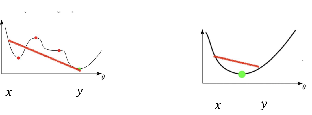 For convex functions, every local minimum = global minimum (linear models + simple loss). Deep networks are non-convex, with many valleys and saddles. Yet, gradient descent still finds good minima.

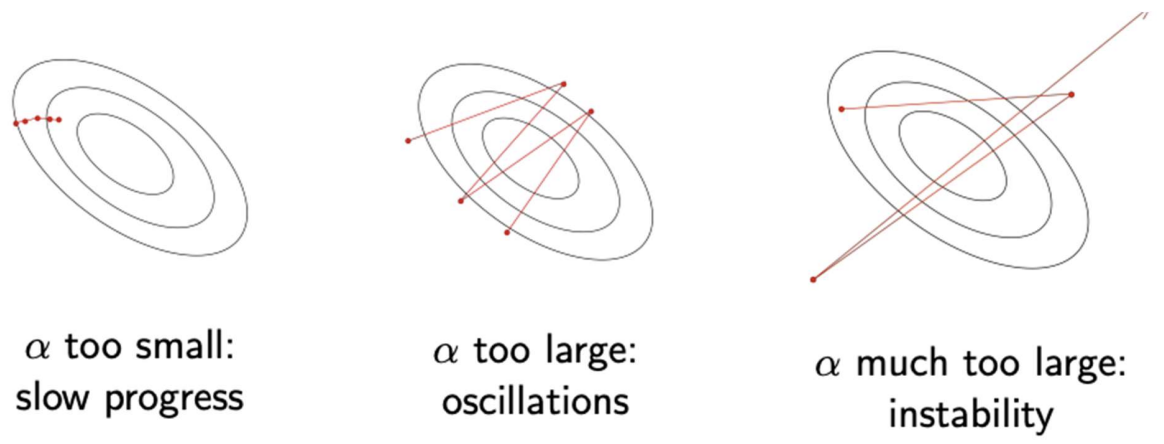
Learning Rate & Schedules

$\alpha$ (step size / learning rate) greatly affects optimization.

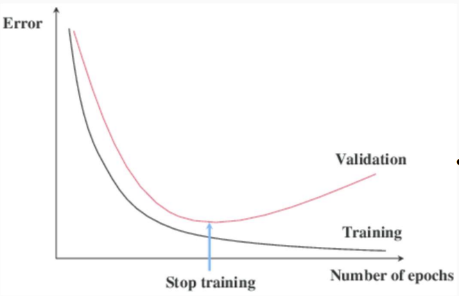
Early Stopping

We should monitor validation loss after each epoch. If it starts increasing while training loss keeps decreasing -> overfitting. We stop training then, and this acts as a regularizer, it prevents the network from memorizing noise.

Epochs

An epoch is a full pass through the entire training dataset. We usually train for 20/50/100 epochs, each time shuffling the data and iterating again.

10,000 samples, batch size of 100, one epoch will be 100 batches ( $100\times100=10000$ ) in early epochs model learns broad patterns, later epochs is fine-tuning but with risk of overfitting.

Inside one epoch:

Training phase:
- We feed mini-batches of training data to model
- After each batch, we
  - compute the training loss (how wrong the model is on that batch)
  - do backpropagation and update the weights
- keep track of average training loss over all batches in this epoch
Validation phase:
- after finishing all batches (i.e one full epoch of training), we pause weight updates
- we feed the validation dataset to the model -> only forward passes, no backprop
- compute the validation loss (how well the model performs on unseen data)

Usually, after 10+ epochs, the training loss keeps decreasing, but the validation loss actually increases -> overfitting (model memorizing training data) -> that’s when early stopping kicks in.

Momentum

To dampen oscillations and noise from noisy gradient, we can use “momentum” to smooth updates by keeping a running average of past gradients.

If successive gradients point in the same direction -> larger steps
If they oscillate -> cancel update -> smoother path $v_t = \beta v_{t-1} + (1-\beta)\nabla_w \mathcal L(w_t)$ $w_{t+1} = w_t - \alpha v_t$ Usually $\beta \approx 0.9$

Adaptive Learning Rates

RMSProp

Tracks a moving average of squared gradients for each parameter, this means that parameters with consistently large gradients get smaller steps. $...$ Defaults: $\rho = 0.9, \alpha = 0.001$

Adam

Combines momentum + RMSProp, it’s the fastest to tune and very robust. Default: $p_1=0.9, p_2 = 0.999, \alpha=0.001$

Second-Order optimization

Rarely used in Deep Learning, as they’re computationally expensive.

Generalization and Optimization Connection

SGD’s inherent noise acts as implicit regularization.

small mini-batches -> noisy gradients -> explore flat minima
flat minima = models that generalize better (robust to small parameter changes) This is why SGD often outperforms deterministic or large-batch training even when both reach low training loss -> this makes it hard to theoretically analyze optimization algorithms in DL.

Batch size and learning rate

When we increase the batch size, each gradient becomes less noisy (more accurate) because it averages over more samples. Therefore, we can safely use a larger learning rate to keep training speed steady. If you instead keep α small, we’ll just train slower.

So we have a rule of thumb (this makes learning rate smaller) $\text{If you multiply batch size by $k$, multiply learning rate by $\sqrt k$}$

for clarity:

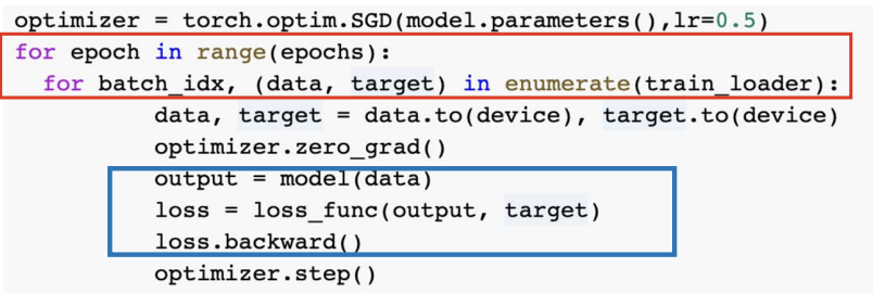
gradients are computed after each batch
the network accumulates all sample losses inside the batch -> averages them -> backpropagates once
then weights are updated once per batch

 for X_batch, Y_batch in dataloader:
   optimizer.zero_grad()
   outputs = model(X_batch)
   loss = criterion(outputs, Y_batch)
   loss.backward()    # compute avg gradient over the batch
   optimizer.step()   # update weights

Distributed and Parallel Optimization

When training on GPUs/TPUs:

Data parallelism (most common): each GPU processes a different mini-batch, then gradients are aggregated
Model parallelism: split layers across devices (used in very large models)
Synchronous SGD: all GPUs compute gradients, sync with a parameter server, update together. The bottleneck is bandwidth for parameter exchange.

Computation costs of training a NN:

Forward / backward pass
- depends on mini-batch size + size of model + efficiency of primitives + hardware
How many iterations/gradient (steps):
- depends on efficiency of optimization algorithm + size of data

Categories